Tree Planning Through The Trees!
Table of Contents:
- 1. Deadline
- 2. Problem Statement
- 3. Environment
- 4. Implementation
- 5. Notes About Test Set
- 6. Submission Guidelines
- 7. Allowed and Disallowed functions
- 8. Collaboration Policy
- 9. Group Contribution
- 10. Acknowledgements
1. Deadline
11:59:59 PM, October 02, 2023.
2. Problem Statement
In this project, you will implement a path and trajectory planning (motion planning), and tune a control stack for a quadrotor to navigate from a start position to a goal position through a pre-mapped or known 3D environment. In the first part of the project 2 AKA project 2a, this will be done in simulation. Fig. 1 shows a block diagram overview of the project.
Download the starter code and environment from here.

3. Environment
The simulation environment is based on Blender which you worked on during P0. Please download the environment and the included starter code from here. The map and the start and goal positions have to be loaded dynamically as described in a text file (more on this in the following sections).
4. Implementation
We will talk about each part in the following sub-sections. Recall that you are implementing four things: (a) A Map/Environment reader and display method, (b) An RRT* path planner to obtain paths from start to goal, (c) A trajectory planner to shorten the paths from RRT* output and make them (dynamically) feasible trajectories, and finally (d) A PID controller to follow the trajectory generated from previous step to navigate from start to goal without collisions. We’ll describe the map file first.
4.1. Map
An example of the environment file format is given below:
# An example environment
# boundary xmin ymin zmin xmax ymax zmax
# block xmin ymin zmin xmax ymax zmax r g b
boundary 0 0 0 45 35 6
block 1.0 1.0 1.0 3.0 3.0 3.0 0 255 0
block 20.0 10.0 0.0 21.0 20.0 6.0 0 0 255
- The format uses # for comments. This is for user reference only.
- The rectangular boundary extents for this environment are
(x0, y0, z0) = (0, 0, 0)(lower left) and(x1, y1, z1) = (45, 35, 6)(upper right). - A block line also specifies the rectangular boundary, and the blocks’ color as a RGB triple with values from 0-255. All values are whitespace delimited and all numerical values are represented as a float.
- All distances (values provided) are in meters.
- Blocks can overlap.
There will be sample files provided to you for testing. This will be available in a folder called sample_maps.
To make life simple, we have made the obstacles cuboidal. In reality, obstacles can be of any shape and size, hence you can think of these rectangular obstacles as the bounding volume of arbitrarily shaped obstacles something that you might obtain from a low resolution occupancy grid mapping algorithm.
Write a simple function to read and display this map in Blender. For the example shown above the environment will look like the image shown in Fig. 1. The start and goal positions are shown as unit red and green spheres respectively. We have shown the environment boundaries with black color and alpha transparency of 0.344 (to enable this, you need to set Blend Mode in Material Properties tab to Alpha Blend). Note that, when you use scale parameter to adjust the block size, it will scale on both directions uniformly (think about what scale value you need to use carefully). Now, bloat the obstacles as shown on the right image in Fig. 2 to perform planning.
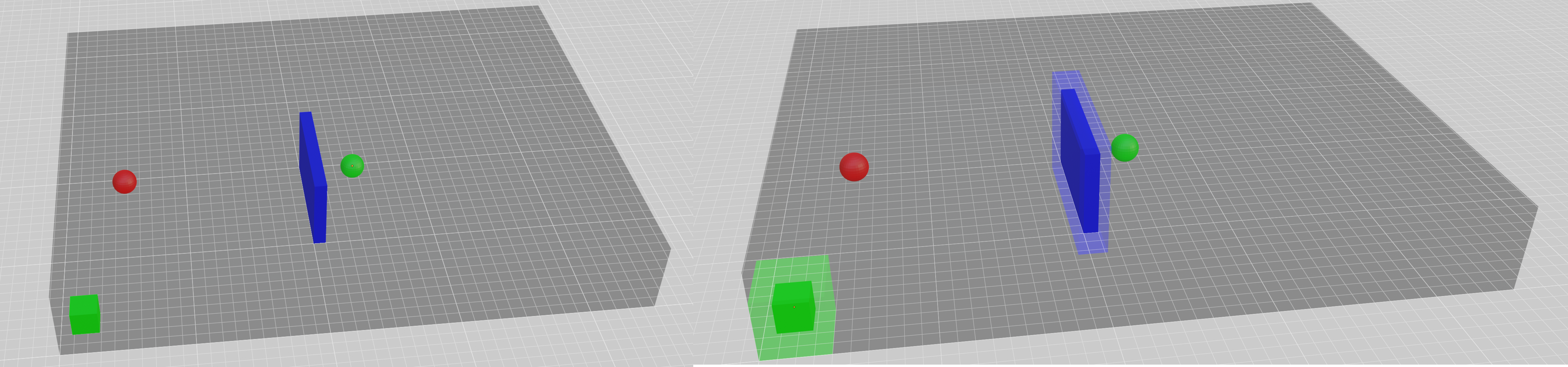
4.2. Path Planner
Now, you’ll write an RRT* global path planner function that takes as input the start position, goal position and the map path from the previous step (You will run your reading and displaying map function from inside the path planner). You are free to use any distance metric in this case. You have complete oracle information (noise free) of the global state (position, velocity, acceleration, orientation and angular velocity) of your robot with respect to the given map. A general rule of thumb is to bloat the obstacles by the size of the robot to avoid collisions as shown in Fig. 2 right side. Write a visualizer in Blender to show exploration paths and nodes you have chosen. You can use simple cylinder objects along with spheres for a great visual tool. You are free to use any third party code for the visualizer here but it has to be in Blender. A simple example of a great package is Blender Plots. Cite the tools you use in your report. Make the visualization functional and pretty! This is super important.

4.3. Trajectory Generation
The path generated in the previous step is not smooth and dynamically feasible as the paths often include sharp turns where the robot will overshoot significantly. In this step, you will convert the waypoints (path) obtained from the previous step into a cubic/quintic spline (3rd/5th order polynomial) though all the waypoints. Optionally, you might want to reduce the path lengths by joining nodes together. This is based on any logic you can come up with. But ensure that no collisions are encountered along the path (See next subsection). Note that you will need to decide on a velocity and acceleration profiles to turn the path from RRT* into a trajectory which will be given by the spline trajectory. Further, you have to decide on the time per segment and the total time the trajectory needs to take. This can be based on simple heuristics such as segment length or you can find an optimal solution using Quadratic Programming as we covered in class.
To summarize, write a function that takes as input a path from RRT* and converts it into a polynomial trajectory as a function of time. You should pre-compute the spline coefficients and avoid fitting polynomial curves in every call of the function.
4.3.1. Collision Handling
Your quadrotor should fly as fast as possible. However, a real quadrotor is not allowed to collide with anything (video). Therefore, we have zero tolerance towards collision - if you collide, you crash, you get zero for that test. For this part, collisions will be counted as if the free space of the robot is an open set; if you are on the boundary of a collision, you are in collision. Note that you have to implement your own collision checker. This is as simple as joining two points with a straight line with some discretization parameter and checking if any of the points lie inside the bloated obstacle blocks. You will use this function not only to stop your code during a collision but also to reject invalid paths in RRT* and trajectory generator. Note that, you start collision check only after you have reached the start point.
As you program your controller, you’ll know how well it works, it will have overshoots. Additionally, trajectory smoothing may also deviate the actual trajectory from the planned path. Therefore, you should make good use of the margin parameter (you can make it bigger than the actual size of the quadrotor) and set your speed carefully (reduce speed and gains to reduce overshoots). Please be aware that the robot is assumed to be a cuboid with a tall vertical height. You should make sure that no part of the robot collides with any obstacles. However, we guarantee that for all the testing maps (you’ll read about this in the test set section), with the specified start and goal locations, there will always be openings that allow cuboid with a width and length of 0.3 m and height of 0.5 m to pass through.
4.4. Controller
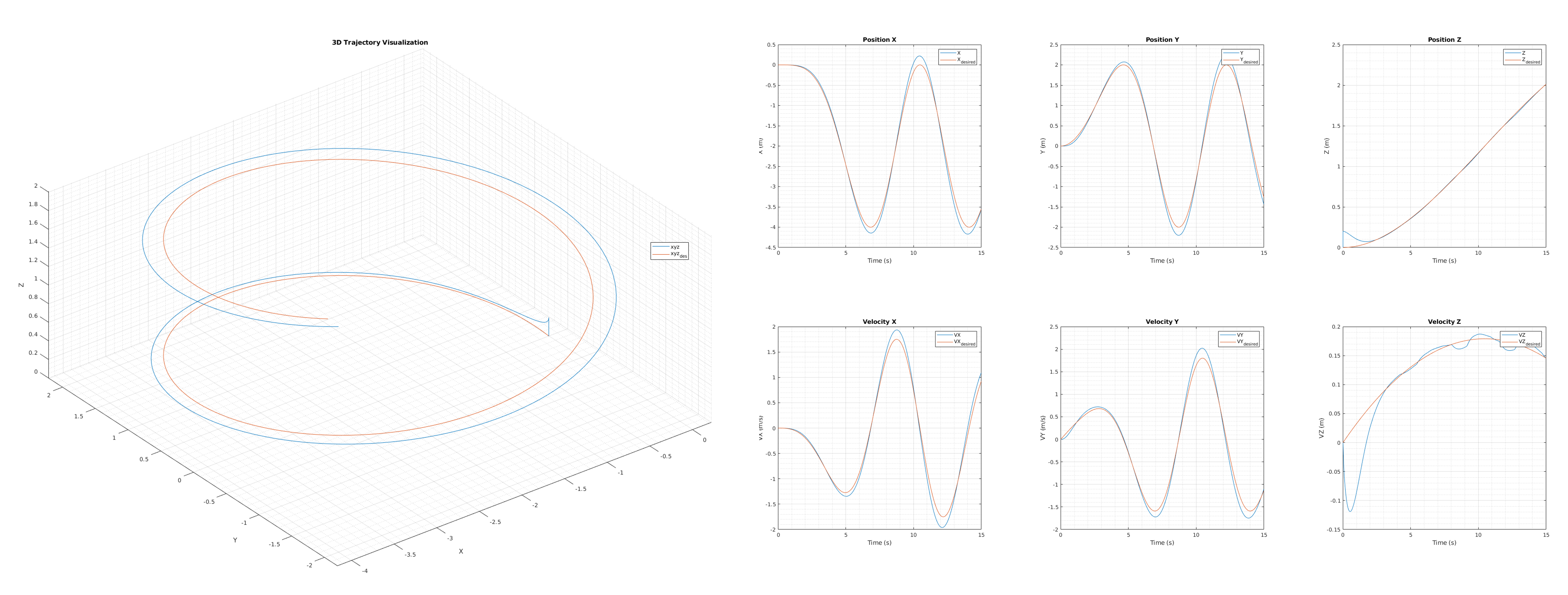
You will then tune a cascaded controller that makes sure that your quadrotor follows the desired trajectory as well as possible. This controller is inspired from the PX4 Stack. The controller takes as input the current state, current time and desired state. In particular, you will tune the outermost position control loop which is a PID controller (3 gains per axis, hence 9 total gains) and the penultimate velocity control loop which is a PID controller (3 gains per axes, hence 9 total gains). Tune your controller on the sample trajectory given in sample_traj folder. Each trajectory file is a .csv file has 9 rows with the rows being px, py, pz, vx, vy, vz, ax, ay, az (position, velocity, acceleration) and each row has number of time steps values. For tuning, utilize the code given in usercode.py’s lines 12-17. Once the controller is tuned, modify this part to take in trajectory waypoints from the previous steps. In this case, plot the desired and actual positions, velocities and 3D trajectories as shown in Fig. 4.
5. Notes About Test Set
A test set will be released 24 hours before the deadline. You can download the test set from here. Your report MUST include the output from both the train and test sets. This will include the maps and the start and goal locations as \((X,Y,Z)\) tuple (you can manually feed these inputs and do not need to write a parsing function).
6. Submission Guidelines
If your submission does not comply with the following guidelines, you’ll be given ZERO credit.
6.1. File tree and naming
Your submission on ELMS/Canvas must be a zip file, following the naming convention YourDirectoryID_p2a.zip. If you email ID is abc@wpi.edu, then your DirectoryID is abc.For our example, the submission file should be named abc_p2a.zip. The file must have the following directory structure. The file to run for your project should be called YourDirectoryID_p2a/Code/main.py. You can have any helper functions in sub-folders as you wish, be sure to index them using relative paths and if you have command line arguments for your Wrapper codes, make sure to have default values too. Attach all the blend files with the main blender file called main.blend in the paths shown below. Please provide detailed instructions on how to run your code in README.md file.
NOTE: Please DO NOT include data in your submission. Furthermore, the size of your submission file should NOT exceed more than 200MB.
The file tree of your submission SHOULD resemble this:
YourDirectoryID_p2a.zip
├── src
|   ├── sample_maps
|   |   ├── map1.txt
|   |   └── map4.txt
|   ├── sample_traj
|   |   └── MP.csv
|   ├── usercode.py
|   ├── main.py
|   ├── Other files and folders
|   └── Any subfolders you want along with files
├── other.blend
├── main.blend
├── Video.mp4
├── Report.pdf
└── README.md
6.2. Report
For each section of the project, explain briefly what you did, and describe any interesting problems you encountered and/or solutions you implemented. You must include the following details in your writeup:
- Your report MUST be typeset in LaTeX in the IEEE Tran format provided to you in the
Draftfolder and should of a conference quality paper. Feel free to use any online tool to edit such as Overleaf or install LaTeX on your local machine. - Plots of desired and actual position and velocity for all the maps in train and test sets as shown in Fig. 4.
- Show a screenshot of the explored tree for all the above cases with the path taken in the tree in red color.
6.3. Video
The video should be a screen capture of your code in action from both an oblique and top view as shown in the video below. Note that a screen capture is not a video recorded from your phone.
7. Allowed and Disallowed functions
Allowed:
- Any functions regarding reading, writing and displaying/plotting
- Basic math utilities
- Any functions for pretty plots and Blender plots
- Quaternion libraries
- Any library that perform transformations between various representations of attitude
- Any code interpolation
- Any least square solver
Disallowed:
- Any function that implements in-part or full RRT*
- Any function that implements in-part or full trajectory polynomial fitting or solving
- Any function that implements in-part or full controller architecture
If you have any doubts regarding allowed and disallowed functions, please drop a public post on Piazza.
8. Collaboration Policy
NOTE: You are STRONGLY encouraged to discuss the ideas with your peers. Treat the class as a big group/family and enjoy the learning experience.
However, the code should be your own, and should be the result of you exercising your own understanding of it. If you reference anyone else’s code in writing your project, you must properly cite it in your code (in comments) and your writeup. For the full honor code refer to the RBE595-F02-ST Fall 2023 website.
9. Group Contribution
If you have any issues/problems with other group members’ work, please send us a private Piazza post right after the submission.
10. Acknowledgements
This fun project is inspired by ENAE788M: Hands-On Autonomous Aerial Robotics at the University of Maryland, College Park and MEAM620: Advanced Robotics at the University of Pennsylvania.