Mini Drone Race -- The Perception Saga!
Table of Contents:
- 1. Deadline
- 2. Problem Statement
- 3. Environment
- 4. Perception Stack
- 5. Testing (Live Demo)
- 6. Submission Guidelines
- 7. Allowed and Disallowed functions
- 8. Tips, Tricks And Hints
- 9. Collaboration Policy
1. Deadline
Live Demo due on 11:59:59 PM, Oct 27, 2023. Everything else due on **11:59:59 PM, Nov 07, 2023.
2. Problem Statement
Drone racing is a fast growing sport that is a great combination of technology and skill. In this sport, professional pilots fly small quadrotors through complex tracks at high speeds (see Fig. 1). Developing a fully autonomous racing drone is difficult due to challenges that span dynamics modeling, onboard perception, localization and mapping, trajectory generation, and optimal control. Recently, Lockheed Martin hosted a competition called AlphaPilot with a whopping 1M USD grand prize.
In this project, you’ll build an autonomy stack to navigate through multiple windows inspired by the AlphaPilot competition. The project is split into two parts: the first part being the perception stack and the second part being the planning, control and integration stack deployed on a real quadrotor.
3. Environment
The track is made of multiple windows with their approximate 3D pose known apriori. In the first stage of project 3, i.e., project 3a, the goal would be to detect/segment the closest window using a deep learning approach and compute it’s 3D pose (See for example Fig. 1 right). More details on the algorithmic parts of the perception stack are explained in the next section.
3.1. Window Locations
An example of the window center location file format is given below:
# An example window environment file
# boundary xmin ymin zmin xmax ymax zmax
# window x y z xdelta ydelta zdelta qw qx qy qz xangdelta yangdelta zangdelta
boundary 0 0 0 45 35 6
window 1 1 1 0.2 0.2 0.2 0.52 0.85 0 0 5 5 5
- The format uses # for comments.
- The rectangular boundary extents for this environment are
(x0, y0, z0) = (0, 0, 0)(lower left) and(x1, y1, z1) = (45, 35, 6)(upper right). - A window line also specifies the center of the window, its approximate pose and variances. All values are whitespace delimited and all numerical values are represented as a float.
- Specifically,
x y zrepresents the approximate center of the window in meters. xdelta ydelta zdeltarepresents the variation in meters that is possible fromx y zvalues (note that this is a uniform distribution on either direction and the probability of the window being outside this is 0).qw qx qy qzrepresents the approximate orientation of the window as a quaternion.xangdelta yangdelta zangdeltarepresents the ZYX Euler angle variation in degrees that is possible from the approximate orientation given (again this is a uniform distribution and the probability of the window being outside this is 0).- No windows can overlap
- Please pay attention to the units.
- The coordinate frame definitions are the same from project 2b.
4. Perception Stack
There are three distinct parts in the perception stack.
4.1. Window Detector
In the first step, implement a deep network to detect/segment the corners of the window or detect/segment the entire window. Here you have a flexibility in the design choice. You can use any network architecture of your choice. Furthermore, your network has to run fast enough on the NVIDIA Orin Nano, so be cognizant of your parameters and architecture.
Your goal would be to build a lightweight neural network that has good accuracy that can be used in the next steps. To accomplish this, you will have to generate windows in simulation (Blender) from different views and backgrounds and scenarios and train your network (See Fig. 2). Be sure to maintain the aspect ratio of the window accurately when generating data for good generalization to the real world (the real windows are printed with no scaling). We will describe the specifications of the window next. The window is almost a square with checkerboard pattern on the edges. Each checkerboard pattern is (highlighted in blue in Fig. 3) of a grid of size \(7 \times 6\) (for X or horizontal and Y or vertical) directions. The distance from checkerboard pattern to either edge is the same dimension as one checkerboard square (yellow highlight in Fig. 3). The WPI logo will always be centered vertically and the PeAR logo will be centered horizontally (however, these can be absent too or be changed to other logos). The window will be the same WPI crimson color (rgb(172, 43, 55)) but can appear different in different lighting. Your data can randomize the viewpoint (or window pose), window lighting, window design with respect to logos, noise, the background among others. The thickness of the window is negligible compared to the height and width of the window. There can be multiple windows in the frame. Also, each window is X-Y symmetric. A high resolution PNG image and the associated PPTX file used to generate the windows are given in the starter package in the textures folder which can be downloaded from here.
4.2. Detection Filtering
Once you have obtained detections/segmentations from the previous step, you might notice that there are multiple windows in the frame, you will need to filter and extract the closest window to fly to. You can use the fact that you approximately know where the windows are in 3D space and project them onto the image plane and find the closest points for filtering. The pixel error between reprojection and the corresponding detection is called re-projection error. Feel free to use this cleverly. See Fig. 4 for an illustration of what this means in 3D.
4.3. Sim2Real
You have trained your neural network in simulation with domain randomization in the hopes of a good sim2real transfer. To test this, you will collect data from your DJI Tello’s camera (you don’t have to fly it if you don’t want to for this part, See Fig. 7 for some sample images). Then run inference on your collected data and inspect to see how well your perception stack works. If it does not work well (as well as you think, it will NOT be perfect, do not worry), go back and change your data generation or use other methods to perform a better sim2real transfer like we talked about in class. You can also reconstruct the entire scene using VisualSfM or nerf-factory or Gaussian Splatting and import the models into Blender to render novel views that look photorealistic. Let your creativity run wild in each of the parts here.
4.4. Pose
In order for the quadrotor to fly through the window in the project 3b, the easiest way is to detect the 3D pose of the window with respect to the current quadrotor position. The first step in doing this is camera calibration.
4.4.1. Calibration
Camera Intrinsic calibration entails with estimating the camera calibration matrix \(K\) which includes the focal length and the principal point and the distortion parameters. You’ll can use the awesome calibration package developed by ETHZ Kalibr or the Matlab’s Calibration toolbox or any other calibration toolbox of your liking to do this. You’ll need either a checkerboard or an april grid to calibrate the camera (See Fig. 5). We found that using the April grid gave us superior results. Feel free to print one (don’t forget to turn off autoscaling or scaling of any sort before printing, you can download these calibration targets from here). Bigger April Grids or checkerboard in general give more accurate results. Large calibration targets from calib.io are located in UH100B (Fig. 5) which you are free to use if you don’t want to print your own. Please be careful with these calibration targets as they are super expensive and hard to replace. For calibration in Blender to test your method in simulation, you can create a “fake” checkerboard/aprilgrid in Blender and calibrate using that :) (See Fig. 5)
You also sometimes need to color calibrate the camera. A simple way to do this is to use a color calibration grid as shown in Fig. 6. It has different standard colors which you’ll match up visually. Another simple way is to capture a scene with “gray” color and make sure that it looks gray. Note that your results will vary based on your monitor’s color calibration as well. Color calibration is important so that the complete dynamic range of all channels are used when converting from Bayer to RGB image. You might not need this step is your data has enough variation such that your neural network models are robust to color variation.
4.4.2. Pose Using PnP
Now that you have the camera calibration matrix \(K\), the detections of window corners from your deep learning + filtering stack on the 2D image, the 3D dimensions of parts of the window (including anything you want to measure), you can estimate the 3D pose \([R, T]\) of the window using the solvePnP function in OpenCV or any other similar functions.
4.4.3. Pose Filtering
Optionally, if your detections are not very accurate, you can filter your pose using a low pass filter, variants of Bayesian filters or a factor graph. Let your creativity run wild in this part.
5. Testing (Live Demo)
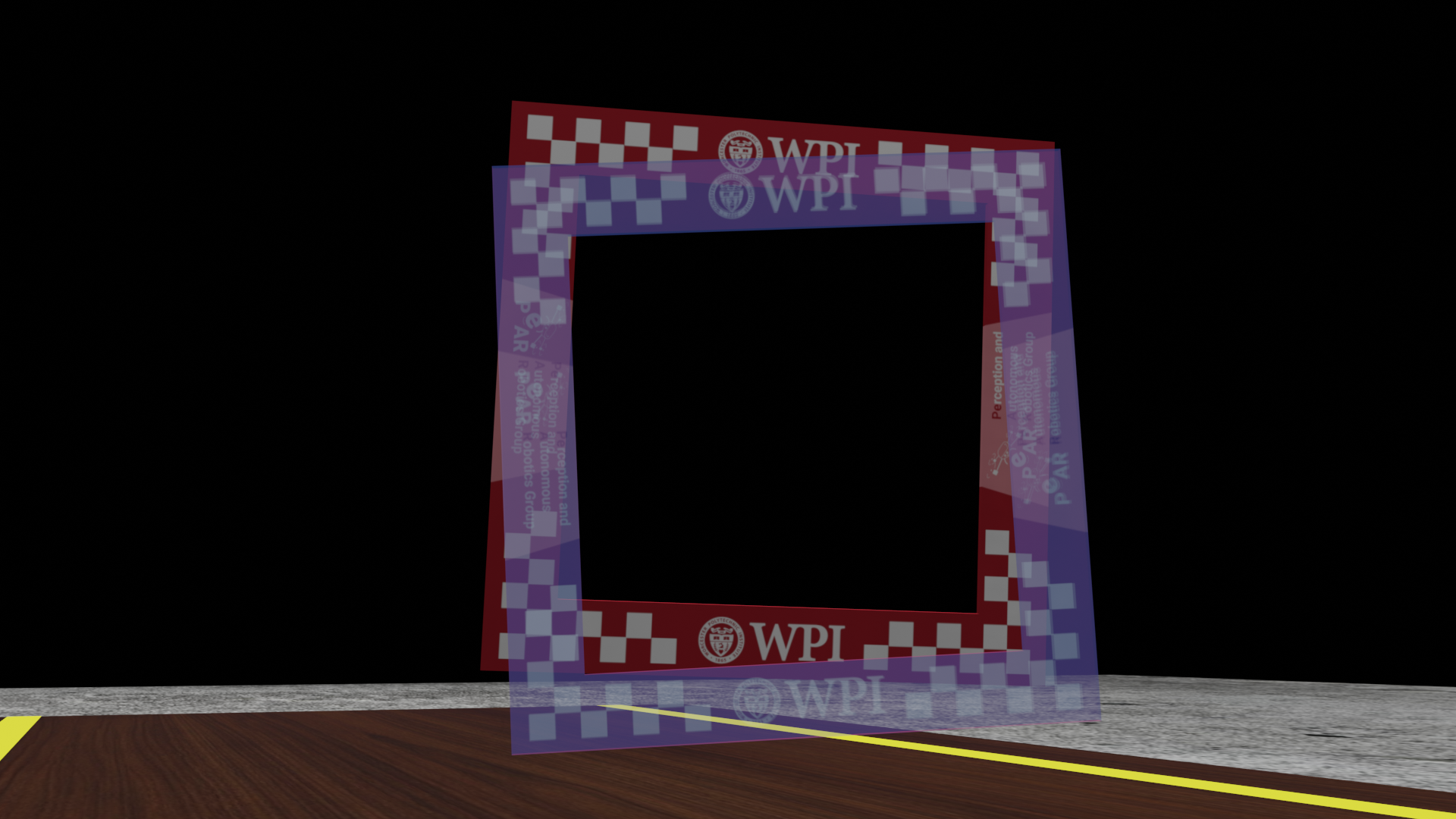
On the day of the deadline, each team will be given a 15 minute slot for demoing their code in action to the instructors. The instructors will hold the quadrotor as they wish and move the drone around with their hand (without flying). The instructors can vary the pose, lighting, color, occlusions, background and so on (See Fig. 7). Note that multiple windows will be present during testing as shown in Fig. 8. You are required to show us the real-time detections along with their estimated 3D pose in Blender (visualization does not have to be real-time, you can save images and run inference, but inference has to be shown real-time). A sample frame of how this can look is shown in Fig. 9. To obtain the highlight as shown in Fig. 9, we set alpha to 0.33, emission color to blue and texture to Window texture.
6. Submission Guidelines
If your submission does not comply with the following guidelines, you’ll be given ZERO credit.
6.1. File tree and naming
Your submission on ELMS/Canvas must be a zip file, following the naming convention YourDirectoryID_p3a.zip. If you email ID is abc@wpi.edu, then your DirectoryID is abc.For our example, the submission file should be named abc_p3a.zip. The file must have the following directory structure. The file to run for your project should be called YourDirectoryID_p3a/Code/Wrapper.py. You can have any helper functions in sub-folders as you wish, be sure to index them using relative paths and if you have command line arguments for your Wrapper codes, make sure to have default values too. Please provide detailed instructions on how to run your code in README.md file.
NOTE: Please DO NOT include data in your submission. Furthermore, the size of your submission file should NOT exceed more than 500MB.
The file tree of your submission SHOULD resemble this:
YourDirectoryID_p3a.zip
├── Code
|   ├── Wrapper.py
|   └── Any subfolders you want along with files
├── Report.pdf
├── Video.mp4
└── README.md
6.2. Report
For each section of the project, explain briefly what you did, and describe any interesting problems you encountered and/or solutions you implemented. You must include the following details in your writeup:
- Your report MUST be typeset in LaTeX in the IEEE Tran format provided to you in the
Draftfolder and should of a conference quality paper. Feel free to use any online tool to edit such as Overleaf or install LaTeX on your local machine.
6.3. Video
Record the data from the live demo in .mp4 format and submit it in the zip file. Make sure to name it as Video.mp4. This video should include the raw footage, the detections (output of the network), Blender visualization of the 3D window pose all stacked side by side. Use the maximum resolution possible here for the best quality.
7. Allowed and Disallowed functions
Allowed:
- Any functions regarding reading, writing and displaying/plotting images in
cv2,matplotlib - Basic math utilities including convolution operations in
numpyandmath - Any functions for pretty plots
- Quaternion libraries
- Any library that perform transformation between various representations of attitude
- Any code for alignment of timestamps
- Any code for data handling, network setup and architecture engineering
- Any code for estimation of 3D poses from 2D images
- Any code for data augmentation and similar functionality
Disallowed:
- Other student’s code in class
If you have any doubts regarding allowed and disallowed functions, please drop a public post on Piazza.
8. Tips, Tricks And Hints
Generating data using Blender can be fun, exciting and equally frustrating at the same time. We are adding some hints, tricks and tips to ease this process. We will do this as a series of question and answers:
1. How do I obtain a segmentation mask of the object in the scene? Can I do this for multiple objects together?
To obtain the segmentation mask, you will use something called the Pass Index in Blender. For each object, go to Object Properties > Relations > Pass Index and set this to a unique number. Now, in your compositing tab, you can use the ID Mask node and look for this Index and write that into a file using the File Output node. You can do this for as many objects as you want as long as they all have a unique Pass Index. This can give you the closest window mask even if you have multiple windows in the scene. Note that this will only work if you have enabled Object Index in View Layer Properties > Passes > Data > Indexes tab.
2. How do I obtain the locations of the corners if I want to train my network to predict corners?
One way is to mark the corners in 3D on the window you crafted. Now, to obtain the image locations on the image, you will use the projection equation to know where each corner lies. This is going to be the most accurate way to obtain corners and you can easily do this for as many points as you want. If you want an easier but less accurate method, here it is: you can create transparent objects (such as a circle or square or anything your heart desires and setting the Material to Principles BSDF shader and Alpha parameter to 0) at the corner locations and have a rigid relation with the window (if you changing window pose). Now assign a unique Pass Index to each of these transparent objects and obtain the mask. However, transparent objects are not rendered in the Pass Index by default. To enable this, you will need to enable Object Properties > Visibility > Holdout for the particular transparent object.
3. What are we trying to predict? Can you talk about the input and output of the network?
The overall goal of the project is to obtain 3D pose of the window from 2D image(s). You are free to use one or more neural networks for any part of the perception stack. You input could be one or more images (temporally) and the output could be either a segmentation mask of the window or some corner points or the 3D pose. These are all design choices you are free to make. Your architecture will vary based on the choice of input and output. Generally, breaking down the problem into sub-problems makes it easier for the network to be trained and generalized from sim2real better.
4. Is it advisable to predict segmentations or the corners for the windows?
Both have pros and cons. Predictions of segmentations might generalize better and you get more data to work with, but this means that you need a better post-processing step. Corner predictions might be harder to train but are easier to interpret at the end. You might want to think about predicting corners more carefully, predicting directly the pixel co-ordinates is generally not advisable due to large numbers, you might want to normalize this with respect to the center of the image (here, image varies from -1 to 1 in each X and Y directions, with (0,0) being in the center). Also, be cognizant of the loss function you are using in both cases. Furthermore, think carefully about how you’ll find the closest window if there are multiple windows in the frame. Also think about how you will find the window if one of the corners or parts of the window are occluded or not detected.
5. How many images do I need to train on?
This depends heavily on the number of parameters in your network. The larger your network, the more data you will need. For example, a 10MB ResNet inspired model needs a minimum of 10K to 100K images with large variations for a good generalized performance. The rule of thumb is that if you increase model size by a factor of \(N\), then you need to increase data amount by \(N^2\). A trick used for better generalization is to train the network in simulation and then fine-tune on real data (this can be as little as 1/10th the amount of simulation data).
6. The data generation is super slow. What can I do?
You can lose photorealism and train in material preview mode. This will not generalize as well but you can train your network first on material preview mode images and then fine-tune on more photo-realistic images. This is generally called curriculum learning.
7. Is there a trick/hack to get photorealistic data faster? Do you have any tips for better sim2real transfer?
One way is to reconstruct the real scene/window in a dense manner using photogrammetry like Visual SfM or newer tools like NeRF or Gaussian Splats. If you have an iPhone or an iPad with a LIDAR sensor, you can use apps like Polycam or LumaAI or Kiri Engine (also works on Android without a LIDAR) ton reconstruct the scene. You can import these point clouds or meshes into Blender to obtain “photo-realistic data” for “free”. This approach coupled with Blender simulation data would most likely lead to a great sim2real generalization.
You can also download an example Blender file to play with the above things from here.
9. Collaboration Policy
NOTE: You are STRONGLY encouraged to discuss the ideas with your peers. Treat the class as a big group/family and enjoy the learning experience.
However, the code should be your own, and should be the result of you exercising your own understanding of it. If you reference anyone else’s code in writing your project, you must properly cite it in your code (in comments) and your writeup. For the full honor code refer to the RBE595-F02-ST Fall 2023 website.