Homework 0 - Alohomora
Table of Contents:
- 1. Due Date
- 2. Phase 1: Shake My Boundary
- 3. Phase 2: Deep Dive on Deep Learning
- 4. Submission Guidelines
- 5. Allowed and Disallowed functions
- 6. Collaboration Policy
- 7. Acknowledgments
1. Due Date
11:59:59PM, Wednesday, Jan 18, 2023. (Individual Submissions) This homework is to be submitted individually. The aim of HW0 is to give you a guage of the quality, expectation and difficulty of this course. You are expected to be able to solve HW0 before the class starts. Remember that HW0 is graded and does count for your final grade. Download starter Code from here.
NOTE: Here is a link to obtain free GPUs for netural network training if you need them.
2. Phase 1: Shake My Boundary
2.1. Introduction
Boundary detection is an important, well-studied computer vision problem. Clearly it would be nice to have algorithms which know where one object transitions to another. But boundary detection from a single image is fundamentally diffcult. Determining boundaries could require object-specific reasoning, arguably making the task hard. A simple method to find boundaries is to look for intensity discontinuities in the image, also known of edges.
Classical edge detection algorithms, including the Canny and Sobel baselines we will compare against, look for these intensity discontinuities. The more recent pb (probability of boundary) boundary detection algorithm significantly outperforms these classical methods by considering texture and color discontinuities in addition to intensity discontinuities. Qualitatively, much of this performance jump comes from the ability of the pb algorithm to suppress false positives that the classical methods produce in textured regions.
In this homework, you will develop a simplified version of pb, which finds boundaries by examining brightness, color, and texture information across multiple scales (different sizes of objects/image). The output of your algorithm will be a per-pixel probability of boundary. Several papers from Berkeley describe their algorithms and how their methods evolved over time. Here we investigate a simplified version of the recent work from this paper. Our simplified boundary detector will still significantly outperform the well regarded Canny and Sobel edge detectors. A qualitative evaluation is carried out against human annotations (ground truth) from a subset of the Berkeley Segmentation Data Set 500 (BSDS500) given to you in YourDirectoryID_hw0/Phase1/BSDS500/ folder.
2.2. Overview
The overview of the algorithm is shown below.
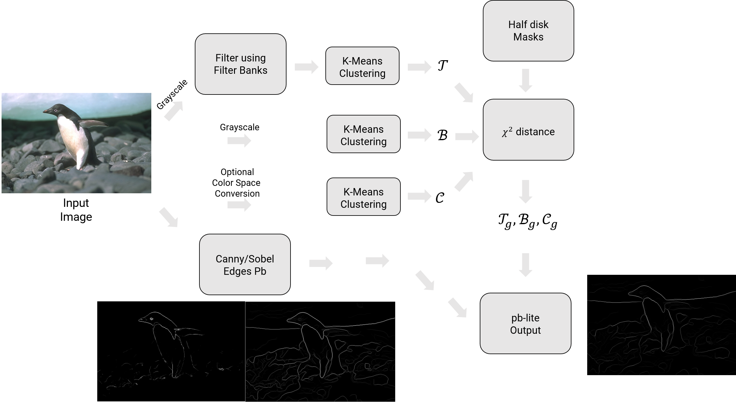
2.3. Filter Banks
The first step of the pb lite boundary detection pipeline is to filter the image with a set of filter banks. We will create three different sets of filter banks for this purpose. Once we filter the image with these filters, we’ll generate a texton map which depicts the texture in the image by clustering the filter responses. Let us denote each filter as \(\mathcal{F}_i\) and texton map as \(\mathcal{T}\).
Let’s talk a little more about filter banks now. Filtering is at the heart of building the low level features we are interested in. We will use filtering both to measure texture properties and to aggregate regional texture and brightness distributions. As we mentioned earlier, we’ll implement three different sets of filters. Let’s talk about each one of them next.
2.3.1. Oriented DoG filters
A simple but effective filter bank is a collection of oriented Derivative of Gaussian (DoG) filters. These filters can be created by convolving a simple Sobel filter and a Gaussian kernel and then rotating the result. Suppose we want \(o\) orientations (from 0 to 360\(^\circ\)) and \(s\) scales, we should end up with a total of \(s \times o\) filters. A sample filter bank of size \(2 \times 16\) with 2 scales and 16 orientations is shown below. We expect you to read up on how these filter banks are generated and implement them. DO NOT use any built-in or third party code for this.

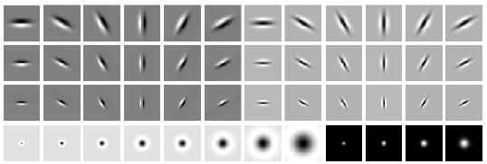
2.3.2. Leung-Malik Filters
The Leung-Malik filters or LM filters are a set of multi scale, multi orientation filter bank with 48 filters. It consists of first and second order derivatives of Gaussians at 6 orientations and 3 scales making a total of 36; 8 Laplacian of Gaussian (LOG) filters; and 4 Gaussians. We consider two versions of the LM filter bank. In LM Small (LMS), the filters occur at basic scales \(\sigma=\{ 1, \sqrt{2}, 2, 2\sqrt{2}\}\). The first and second derivative filters occur at the first three scales with an elongation factor of 3, i.e., (\(\sigma_x = \sigma\) and \(\sigma_y = 3\sigma_x\)). The Gaussians occur at the four basic scales while the 8 LOG filters occur at \(\sigma\) and \(3\sigma\). For LM Large (LML), the filters occur at the basic scales \(\sigma=\{\sqrt{2}, 2, 2\sqrt{2}, 4 \}\). You need to implement both LMS and LML filter banks and DO NOT use any built-in or third party code for this. The filter bank is shown below. More details about these filters can be found here.
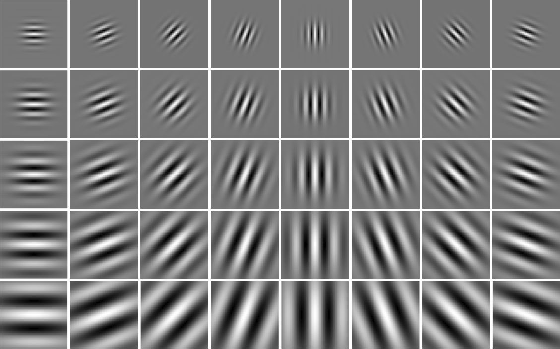
2.3.3. Gabor Filters
Gabor Filters are designed based on the filters in the human visual system. A gabor filter is a gaussian kernel function modulated by a sinusoidal plane wave. More details can be found on the Wikipedia page. Implement any number of Gabor filters and DO NOT use any built-in or third party code for this. A sample of gabor filters is shown below.
2.4. Texton Map \(\mathcal{T}\)
Filtering an input image with each element of your filter bank (you can have a lot of them from all the three filter banks you implemented) results in a vector of fillter responses centered on each pixel. For instance, if your filter bank has \(N\) filters, you’ll have \(N\) filter responses at each pixel. A distribution of these \(N\)-dimensional filter responses could be thought of as encoding texture properties. We will simplify this representation by replacing each \(N\)-dimensional vector with a discrete texton ID. We will do this by clustering the filter responses at all pixels in the image in to \(K\) textons using kmeans (feel free to use Scikit learn’s sklearn.cluster.KMeans function or implement your own). Each pixel is then represented by a one dimensional, discrete cluster ID instead of a vector of high-dimensional, real-valued filter responses (this process of dimensionality reduction from \(N\) to 1 is called “Vector Quantization”). This can be represented with a single channel image with values in the range of \([1, 2, 3, \cdots , K]\). \(K =
64\) seems to work well but feel free to experiment. To visualize the texton map, you can try the matplotlib.pyplot.imshow command with proper scaling arguments.
2.5. Brightness Map \(\mathcal{B}\)
The concept of the brightness map is as simple as capturing the brightness changes in the image. Here, again we cluster the brightness values using kmeans clustering (grayscale equivalent of the color image) into a chosen number of clusters (16 clusters seems to work well, feel free to experiment). We call the clustered output as the brightness map \(\mathcal{B}\).
2.6. Color Map \(\mathcal{C}\)
The concept of the color map is to capture the color changes or chrominance content in the image. Here, again we cluster the color values (you have 3 values per pixel if you have RGB color channels) using kmeans clustering (feel free to use alternative color spaces like YCbCr, HSV or Lab) into a chosen number of clusters (16 clusters seems to work well, feel free to experiment). We call the clustered output as the color map \(\mathcal{C}\). Note that you can also cluster each color channel seprarately here. Feel free to experiment with different methods.
2.7. Texture, Brightness and Color Gradients \(\mathcal{T}_g, \mathcal{B}_g, \mathcal{C}_g\)
To obtain \(\mathcal{T}_g, \mathcal{B}_g, \mathcal{C}_g\), we need to compute differences of values across different shapes and sizes. This can be achieved very efficiently by the use of Half-disc masks.
Let us first implement these Half-disc masks. Here’s an image of how these Half-disc masks look.
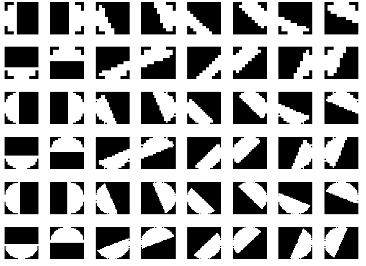
The half-disc masks are simply (pairs of) binary images of half-discs. This is very important because it will allow us to compute the \(\chi^2\) (chi-square) distances (finally obtain values of \(\mathcal{T}_g, \mathcal{B}_g, \mathcal{C}_g\)) using a filtering operation, which is much faster than looping over each pixel neighborhood and aggregating counts for histograms. Forming these masks is quite trivial. A sample set of masks (8 orientations, 3 scales) is shown in Fig. 4.
NOTE: The filter banks and masks only need to be defined once and then they will be used on all images.
\(\mathcal{T}_g, \mathcal{B}_g, \mathcal{C}_g\) encode how much the texture, brightness and color distributions are changing at a pixel. We compute \(\mathcal{T}_g, \mathcal{B}_g, \mathcal{C}_g\) by comparing the distributions in left/right half-disc pairs (opposing directions of filters at same scale, in Fig. 4, the left/right pairs are shown one after another, these are easy to create as you have control over the angle) centered at a pixel. If the distributions are the similar, the gradient should be small. If the distributions are dissimilar, the gradient should be large. Because our half-discs span multiple scales and orientations, we will end up with a series of local gradient measurements encoding how quickly the texture or brightness distributions are changing at different scales and angles.
We will compare texton, brightness and color distributions with the \(\chi^2\) measure. The \(\chi^2\) distance is a frequently used metric for comparing two histograms. \(\chi^2\) distance between two histograms \(g\) and \(h\) with the same binning scheme is defined as follows
\[\chi^2(g,h) = \frac{1}{2} \sum_{i=1}^K {\frac{(g_i - h_i)^2}{g_i + h_i}}\]here, \(K\) indexes though the bins. Note that the numerator of this expression is simply the sum of squared difference between histogram elements. The denominator adds a “soft” normalization to each bin so that less frequent elements still contribute to the overall distance.
To effciently compute \(\mathcal{T}_g, \mathcal{B}_g, \mathcal{C}_g\), filtering can used to avoid nested loops over pixels. In addition, the linear nature of the formula above can be exploited. At a single orientation and scale, we can use a particular pair of masks to aggregate the counts in a histogram via a filtering operation, and compute the \(\chi^2\) distance (gradient) in one loop over the bins according to the following outline:
chi_sqr_dist = img*0
for i = 1:num_bins
	tmp = 1 where img is in bin i and 0 elsewhere
	g_i = convolve tmp with left_mask
	h_i = convolve tmp with right_mask
	update chi_sqr_dist
end
The above procedure should generate a 2D matrix of gradient values. Simply repeat this for all orientations and scales, you should end up with a 3D matrix of size \(m \times n \times N\), where \((m,n)\) are dimensions of the image and \(N\) is the number of filters.
2.8. Sobel and Canny baselines
canny_pb and sobel_pb baseline outputs are provided in YourDirectoryID_hw0/Phase1/BSDS500/CannyBaseline/ and YourDirectoryID_hw0/Phase1/BSDS500/SobelBaseline/ respectively.
2.9. Pb-lite Output
The final step is to combine information from the features with a baseline method (based on Sobel or Canny edge detection or an average of both) using a simple equation
\[PbEdges = \frac{(\mathcal{T}_g + \mathcal{B}_g +\mathcal{C}_g)}{3}\odot (w_1*cannyPb + w_2*sobelPb)\]Here, \(\odot\) is the Hadamard product operator. A simple choice for \(w_1\) and \(w_2\) would be 0.5 (they have to sum to 1). However, one could make these weights dynamic.
The magnitude of the features represents the strength of boundaries, hence, a simple mean of the feature vector at location \(i\) should be somewhat proportional to pb. Of course, fancier ways to combine the features can be explored for better performance. As a starting point, you can simply use an element-wise product of the baseline output and the mean feature strength to form the final pb value, this should work reasonably well.
3. Phase 2: Deep Dive on Deep Learning
3.1. Problem Statement
For phase 2 of this homework, you’ll be implementing multiple neural network architectures and comparing them on various criterion like number of parameters, train and test set accuracies and provide detailed analysis of why one architecture works better than another one.
3.2. Dataset
CIFAR-10 is a dataset consisting of 60000, 32\(\times\)32 colour images in 10 classes, with 6000 images per class. There are 50000 training images and 10000 test images. More details about the datset can be found here.
Sample images from each class of the CIFAR-10 dataset is shown below:
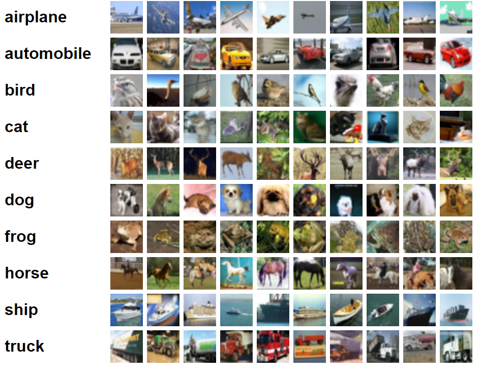
A randomized version of the CIFAR-10 dataset with 50000 training images and 10000 test images is given to you in the CIFAR10 folder of your hw0.zip file. CIFAR10 has two subfolders Train and Test for training and testing images respectively stored in .png format for ease of viewing and loading.
3.3. Train your first neural network
The task in this part is to train a convolutional neural network on PyTorch for the task of classification. The input is a single CIFAR-10 image and the output is the probabilities of 10 classes. The starter code given to you has Train.py file for training and Test.py for testing. Fill in the following files with respective details.
Optimizervalue with various parameters inTrainOperationfunction inTrain.pyfile (Feel free to use any architecture and optimizer for this part)loss functioninTrainOperationfunction inTrain.pyfile (You’ll be using cross entropy loss for training)- Network architecture in
CIFAR10Modelfunction inNetwork/Network.pyfile (We recommend using thetorch.nnAPI for implementing layers)
If you are super new to machine learning and deep learning, there are a lot of resources online to learn how to program a simple neural network, tune hyperparameters for CIFAR-10. A good starting point is the official PyTorch tutorial and this great tutorial by sentdex. If you are new to deep learning, we recommend reading up basics from CS231n course offered by Stanford University here.
The starter code given to you has Tensorboard code snippets built-in and displays training accuracy per batch and the loss value. You can run TensorBoard using the following command tensorboard --logdir=path/to/log-directory.
Report the train accuracy over epochs (training accuracy over the whole train dataset not just minibatches as given to you!, you need to implement this), test accuracy over epochs (test accuracy over the whole test dataset!, you need to implement this), number of parameters in your model (code for this can be found in Test.py and snippet is also given next), plot of loss value over epochs (not over minibatches as given to you!, you need to sum up loss values for all iterations of an epoch to achieve this), your architecture, other hyperparameters chosen such as optimizer, learning rate and batch size. Also present a confusion matrix for both training and testing data (code in Test.py).
You can use the following snippet of code to obtain the number of parameters in your model. More details can be found here.
for name, param in model.named_parameters():
    if param.requires_grad:
        print name, param.data
Congratulations! You’ve just successfully trained your first neural network. A pro tip is to use Netron to visualize your network, this will massively help in debugging and has a coll visualization that you can include in your report.
3.4. Improving Accuracy of your neural network
Now that we have a baseline neural network working, let’s try to improve the accuracy by doing simple tricks.
- Standardize your data input if you haven’t already. There are a lot of ways to do this. Feel free to search for different methods. A simple way is to scale data from [0,255] to [-1,1]. Fill in this code in the
GenerateBatchfunction ofTrain.pyfile. - Decay your learning rate as you train or Increase your batch size as you train. Refer to this paper for more details.
- Augment your data to artificially make your dataset larger. Refer to this link nice data augmentation functions.
- Add Batch Normalization between layers.
- Change the hyperparameters in your architecture such as number of layers, number of neurons.
Now, feel free to implement as many of these as possible and present a detailed analysis of your findings as before. Present the same details as before, train and test accuracy over epochs, number of parameters in your model, loss value over epochs, your architecture and details of other tricks you employed. Also present a confusion matrix for both training and testing data (code in Test.py).
3.5. ResNet, ResNeXt, DenseNet
Now, let’s make the architectures more efficient in-terms of memory usage (number of parameters), computation (number of operations) and accuracy. Read up the concepts from ResNet, ResNeXt and DenseNet and implement all of these architectures with the parameters of your choice. DO NOT use any built-in or third party code for this apart from the API functions mentioned before. Fill in the code in Network/Network.py as different functions.
Present a detailed analysis of all these architectures with your earlier findings. Present the same details as before, train and test accuracy over epochs, number of parameters in your model, loss value over epochs, your architecture and details of other tricks you employed. Also present a confusion matrix for both training and testing data (code in Test.py).
4. Submission Guidelines
If your submission does not comply with the following guidelines, you’ll be given ZERO credit.
4.1. Starter Code
Download the Starter Code for both Phase 1 and Phase 2 from here.
4.2. File tree and naming
Your submission on ELMS/Canvas must be a zip file, following the naming convention YourDirectoryID_hw0.zip. If you email ID is abc@wpi.edu, then your DirectoryID is abc. For our example, the submission file should be named abc_hw0.zip. The file must have the following directory structure because we might be autograding assignments. The file to run for your project should be called YourDirectoryID_hw0/Phase1/Code/Wrapper.py for Phase 1; YourDirectoryID_hw0/Phase2/Code/Train.py and YourDirectoryID_hw0/Phase2/Code/Test.py for Phase 2 or HW0Phase1AndPhase2Notebook.ipynb if you are using a Notebook. You can have any helper functions in sub-folders as you wish, be sure to index them using relative paths and if you have command line arguments for your Wrapper codes, make sure to have default values too. Please provide detailed instructions on how to run your code in README.md file.
NOTE: Please DO NOT include data in your submission.
The file tree of your submission SHOULD resemble this:
YourDirectoryID_hw0.zip
|   Phase1
|   ├── Code
|   |   ├── Wrapper.py
|   |   ├── Any subfolders you want along with files
|   Phase2
|   ├── Code
|   |   ├── Train.py
|   |   ├── Test.py
|   |   ├── Any subfolders you want along with files
|   └── HW0Phase1AndPhase2Notebook.ipynb
├── Report.pdf
└── README.md
4.3. Report
For each section of the homework, explain briefly what you did, and describe any interesting problems you encountered and/or solutions you implemented. You must include the following details in your writeup:
- Your report MUST be typeset in LaTeX in the IEEE Tran format provided to you in the
Draftfolder and should of a conference quality paper.
Phase 1
- Present a detailed explanation for Phase 1 along with outputs images of the filter banks (all of them with appropriate labels), \(\mathcal{T}, \mathcal{B}, \mathcal{C}, \mathcal{T}_g, \mathcal{B}_g, \mathcal{C}_g\), sobel and canny baselines and the final pb-lite output for all the images provided. Provide a detailed analysis of the approach and why you think it’s better than the sobel and canny baselines.
Phase 2
- Section 3.3
- Plot of
Train_AccuracyoverEpochs(Not over Iterations) - Plot of
Test_AccuracyoverEpochs(Not over Iterations) - Number of Parameters in your model
- Plot of
lossoverEpochs(Not over Iterations) - An Image of the architecture (a snapshot of tensorboard graph would work, if it has meaningful names)
- Optimizer chosen with the specific hyperparameters (learning rate etc.)
- Batch size chosen
- Confusion Matrix of the trained model on training data
- Confusion Matrix of the trained model on testing data
- Plot of
- Section 3.4
- Plot of
Train_AccuracyoverEpochs(Not over Iterations) - Plot of
Test_AccuracyoverEpochs(Not over Iterations) - Number of Parameters in your model
- Plot of
lossoverEpochs(Not over Iterations) - An Image of the architecture (a snapshot of tensorboard graph would work, if it has meaningful names)
- Optimizer chosen with the specific hyperparameters (learning rate etc.)
- Batch size chosen
- Confusion Matrix of the trained model on training data
- Confusion Matrix of the trained model on testing data
- A detailed analysis of all the tricks used
- Plot of
- Section 3.5
For each Architecture:
- Plot of
Train_AccuracyoverEpochs(Not over Iterations) - Plot of
Test_AccuracyoverEpochs(Not over Iterations) - Number of Parameters in your model
- Plot of
lossoverEpochs(Not over Iterations) - An Image of the architecture (a snapshot of tensorboard graph would work, if it has meaningful names)
- Optimizer chosen with the specific hyperparameters (learning rate etc.)
- Batch size chosen
- Confusion Matrix of the trained model on training data
- Confusion Matrix of the trained model on testing data
- Plot of
- Compare all the sections (3.3 - 3.5) and analyze why one works better than the other. Finally, present a comparison of number of parameters, final train and final test accuracy, inference run-time (test time per image after the PyTorch graph is setup) and other competences of your choice in a tabular form for Sections 3.3, 3.4 and 3.5.
5. Allowed and Disallowed functions
Allowed:
- Any functions regarding reading, writing and displaying/plotting images in
cv2,matplotlib - Basic math utilities including convolution operations in
numpyandmath KMeansclustering fromsklearnorscipytorch.nnAPI for implementing network architecturetorchvision.transformfor data augmentation- Any functions for pretty plots
Disallowed:
- Any function that generates
gaussianor any otherfilter/ filter banks - Any third party code for implementing architecture or augmentation
Kerasor any other layer API or built-in models for ResNet, ResNeXt or DenseNet
If you have any doubts regarding allowed and disallowed functions, please drop a public post on Piazza.
6. Collaboration Policy
NOTE: You are STRONGLY encouraged to discuss the ideas with your peers. Treat the class as a big group/family and enjoy the learning experience.
However, the code should be your own, and should be the result of you exercising your own understanding of it. If you reference anyone else’s code in writing your project, you must properly cite it in your code (in comments) and your writeup. For the full honor code refer to the RBE/CS549 Spring 2023 website.
7. Acknowledgments
This fun homework was inspired by a similar project in University of Maryland’s CMSC733 (Classical and Deep Learning Approaches for Geometric Computer Vision) and Brown University’s CS 143 (Introduction to Computer Vision).