Buildings built in minutes - SfM and NeRF
Table of Contents:
- 1. Deadline
- 2. Introduction
- 3. Dataset for Classical SfM
- 4. Phase 1: Traditional Approach
- 5. Putting the pipeline together
- 6. Phase 2: Deep Learning Approach
- 7. Submission Guidelines
- 8. Extra Credit
- 9. Collaboration Policy
- 10. Acknowledgments
1. Deadline
11:59:59 PM, Mar 12, 2023. This project is to be done in groups of 2.
2. Introduction
We have been playing with images for so long, mostly in 2D scene. Recall project 1 where we stitched multiple images with about 30-50% common features between a couple of images. Now let’s learn how to reconstruct a 3D scene and simultaneously obtain the camera poses of a monocular camera w.r.t. the given scene. This procedure is known as Structure from Motion (SfM). As the name suggests, you are creating the entire rigid structure from a set of images with different view points (or equivalently a camera in motion). A few years ago, Agarwal et. al published Building Rome in a Day in which they reconstructed the entire city just by using a large collection of photos from the Internet. Ever heard of Microsoft Photosynth? Fascinating? isn’t it!? There are a few open source SfM algorithm available online like VisualSFM. Try them!
Let’s learn how to recreate such algorithm. There are a few steps that collectively form SfM:
- Feature Matching and Outlier rejection using RANSAC
- Estimating Fundamental Matrix
- Estimating Essential Matrix from Fundamental Matrix
- Estimate Camera Pose from Essential Matrix
- Check for Cheirality Condition using Triangulation
- Perspective-n-Point
- Bundle Adjustment
3. Dataset for Classical SfM
You are going to run classical SfM algorithm on the data provided here. The data given to you are a set of 5 images of Unity Hall at WPI (See Fig. 1), using a Samsung S22 Ultra’s primary camera at f/1.8 aperture, ISO 50 and 1/500 sec shutter speed.

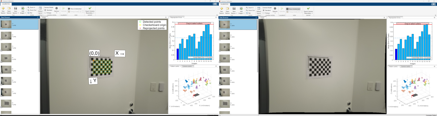
The camera is calibrated after resizing using a Radial-Tangential model with 2 radial parameters and 1 tangential parameter using the MATLAB R2022a’s Camera Calibrator Application (See Fig. 2).
The images provided are already distortion corrected and resized to \(800 \times 600 px.\). Since Structure from Motion relies heavily on good features and their matching, keypoint matching (SIFT keypoints and descriptors are used for high robustness) data is also provided in the same folder for pairs of images. The data folder contains 4 matching files named matching*.txt where * refers to numbers from 1 to 5. For eg., matching3.txt contains the matching between the third image and images that come after (such as images 4 and 5), i.e., \(\mathcal{I}_3 \leftrightarrow \mathcal{I}_4, \mathcal{I}_3 \leftrightarrow \mathcal{I}_5\). This is the reason image 5 does not have a text file.
The file format of the matching file is described next. Each matching file is formatted as follows for the i th matching file:
nFeatures: (the number of feature points of the \(i^{th}\) image - each following row specifies matches across images given a feature location in the \(i^{th}\) image.)
Each Row: (the number of matches for the \(j^{th}\) feature) (Red Value) (Green Value) (Blue Value) (\(u_{\texttt{current image}}\)) (\(v_{\texttt{current image}}\)) (image id) (\(u_{\texttt{image id image}}\)) (\(v_{\texttt{image id image}}\)) (image id) (\(u_{\texttt{image id image}}\)) (v_{image id image}) …
An example of matching1.txt is given below:
nFeatures: 3930
2 255 255 255 5.08304 116.978 3 49.0748 166.783
3 79 71 51 7.15528 197.921 2 11.255 225.237 5 259.685 103.719
The images are taken at \(4000 \times 3000 px.\) but are resized to \(800 \times 600 px.\) before the camera intrinsic parameters \(K\) are estimated which are given in calibration.txt file. You will program this full pipeline guided by the functions described in following sections.
4. Classical Approach to the SfM problem
4.1. Feature Matching, Fundamental Matrix and RANSAC
We have already learned about keypoint matching using SIFT keypoints and descriptors (Recall Project 1: Panorama Stitching). It is important to refine the matches by rejecting outline correspondence. Before rejecting the correspondences, let us first understand what Fundamental matrix is!
4.2. Estimating Fundamental Matrix
The fundamental matrix, denoted by \(F\), is a \(3\times 3\) (rank 2) matrix that relates the corresponding set of points in two images from different views (or stereo images). But in order to understand what fundamental matrix actually is, we need to understand what epipolar geometry is! The epipolar geometry is the intrinsic projective geometry between two views. It only depends on the cameras’ internal parameters (\(K\) matrix) and the relative pose i.e. it is independent of the scene structure.
4.2.1. Epipolar Geometry
Let’s say a point \(\mathbf{X}\) in the 3D-space (viewed in two images) is captured as \(\mathbf{x}\) in the first image and \(\mathbf{x'}\) in the second. Can you think how to formulate the relation between the corresponding image points \(\mathbf{x}\) and \(\mathbf{x'}\)? Consider Fig. 2. Let \(\mathbf{C}\) and \(\mathbf{C'}\) be the respective camera centers which forms the baseline for the stereo system. Clearly, the points \(\mathbf{x}\), \(\mathbf{x'}\) and \(\mathbf{X}\) (or \(\mathbf{C}\), \(\mathbf{C'}\) and \(\mathbf{X}\)) are coplanar i.e. \(\mathbf{\overrightarrow{Cx}}\cdot \left(\mathbf{\overrightarrow{CC'}}\times\mathbf{\overrightarrow{C'x'}}\right)=0\) and the plane formed can be denoted by \(\pi\). Since these points are coplanar, the rays back-projected from \(\mathbf{x}\) and \(\mathbf{x'}\) intersect at \(\mathbf{X}\). This is the most significant property in searching for a correspondence.
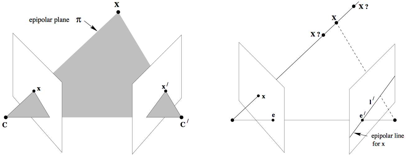

Now, let us say that only \(\mathbf{x}\) is known, not \(\mathbf{x'}\). We know that the point \(\mathbf{x'}\) lies in the plane \(\pi\) which is governed by the camera baseline \(\mathbf{CC'}\) and \(\mathbf{\overrightarrow{Cx}}\). Hence the point \(\mathbf{x'}\) lies on the line of intersection of \(\mathbf{l'}\) of \(\pi\) with the second image plane. The line \(\mathbf{l'}\) is the image in the second view of the ray back-projected from \(\mathbf{x}\). This line \(\mathbf{l'}\) is called the epipolar line corresponding to \(\mathbf{x}\). The benefit is that you don’t need to search for the point corresponding to \(\mathbf{x}\) in the entire image plane as it can be restricted to the \(\mathbf{l'}\).
- Epipole is the point of intersection of the line joining the camera centers with the image plane. (see \(\mathbf{e}\) and \(\mathbf{e'}\) in the Fig. 2(a))
- Epipolar plane is the plane containing the baseline.
- Epipolar line is the intersection of an epipolar plane with the image plane. All the epipolar lines intersect at the epipole.
4.2.2. The Fundamental Matrix \(\mathbf{F}\)
The \(\mathbf{F}\) matrix is only an algebraic representation of epipolar geometry and can both geometrically (constructing the epipolar line) and arithmetically. (See derivation (Page 242)) (Fundamental Matrix Song) As a result, we obtain: \(\mathbf{x}_i'^{\ \mathbf{T}}\mathbf{F} \mathbf{x}_i = 0\), where \(i=1,2,\dots,m.\) This is known as epipolar constraint or correspondence condition (or Longuet-Higgins equation). Since, \(\mathbf{F}\) is a \(3\times3\) matrix, we can set up a homogeneous linear system with 9 unknowns:
\[\begin{bmatrix} x'_i & y'_i & 1 \end{bmatrix} \begin{bmatrix}f_{11} & f_{12} & f_{13} \\ f_{21} & f_{22} & f_{23} \\ f_{31} & f_{32} & f_{33} \end{bmatrix} \begin{bmatrix} x_i \\ y_i \\ 1 \end{bmatrix} = 0\]\(\begin{equation}x_i x'_i f_{11} + x_i y'_i f_{21} + x_i f_{31} + y_i x'_i f_{12} + y_i y'_i f_{22} + y_i f_{32} + x'_i f_{13} + y'_i f_{23} + f_{33}=0\end{equation}\)
Simplifying for \(m\) correspondences,
\[\begin{bmatrix} x_1 x'_1 & x_1 y'_1 & x_1 & y_1 x'_1 & y_1 y'_1 & y_1 & x'_1 & y'_1 & 1 \\ \vdots & \vdots & \vdots & \vdots & \vdots & \vdots & \vdots & \vdots & \vdots \\ x_m x'_m & x_m y'_m & x_m & y_m x'_m & y_m y'_m & y_m & x'_m & y'_m & 1 \end{bmatrix}\begin{bmatrix} f_{11} \\ f_{21} \\ f_{31} \\ f_{12} \\ f_{22} \\ f_{32} \\ f_{13} \\f_{23} \\ f_{33}\end{bmatrix} = 0\]How many points do we need to solve the above equation? Think! Twice! Remember homography, where each point correspondence contributes two constraints? Unlike homography, in \(\mathbf{F}\) matrix estimation, each point only contributes one constraints as the epipolar constraint is a scalar equation. Thus, we require at least 8 points to solve the above homogenous system. That is why it is known as Eight-point algorithm.
With \(N \geq 8\) correspondences between two images, the fundamental matrix, \(F\) can be obtained as: By stacking the above equation in a matrix \(A\), the equation \(Ax=0\) is obtained. This system of equation can be answered by solving the linear least squares using Singular Value Decomposition (SVD) as explained in the Math module. When applying SVD to matrix \(\mathbf{A}\), the decomposition \(\mathbf{USV^T}\) would be obtained with \(\mathbf{U}\) and \(\mathbf{V}\) orthonormal matrices and a diagonal matrix \(\mathbf{S}\) that contains the singular values. The singular values \(\sigma_i\) where \(i\in[1,9], i\in\mathbb{Z}\), are positive and are in decreasing order with \(\sigma_9=0\) since we have 8 equations for 9 unknowns. Thus, the last column of \(\mathbf{V}\) is the true solution given that \(\sigma_i\neq 0 \ \forall i\in[1,8], i\in\mathbb{Z}\). However, due to noise in the correspondences, the estimated \(\mathbf{F}\) matrix can be of rank 3 i.e. \(\sigma_9\neq0\). So, to enforce the rank 2 constraint, the last singular value of the estimated \(\mathbf{F}\) must be set to zero. If \(F\) has a full rank then it will have an empty null-space i.e. it won’t have any point that is on entire set of lines. Thus, there wouldn’t be any epipoles. See Fig. 3 for full rank comparisons for \(F\) matrices.

In MATLAB, you can use svd to solve \(\mathbf{x}\) from \(\mathbf{Ax}=0\)
[U, S, V] = svd(A);
x = V(:, end);
F = reshape(x, [3,3])';
To sumarize, write a function EstimateFundamentalMatrix.py that linearly estimates a fundamental matrix \(F\), such that \(x_2^T F x_1 = 0\). The fundamental matrix can be estimated by solving the linear least squares \(Ax=0\).
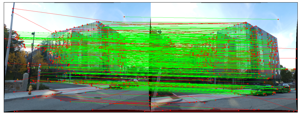
4.2.3. Match Outlier Rejection via RANSAC
Since the point correspondences are computed using SIFT or some other feature descriptors, the data is bound to be noisy and (in general) contains several outliers. Thus, to remove these outliers, we use RANSAC algorithm (Yes! The same as used in Panorama stitching!) to obtain a better estimate of the fundamental matrix. So, out of all possibilities, the \(\mathbf{F}\) matrix with maximum number of inliers is chosen. Below is the pseduo-code that returns the \(\mathbf{F}\) matrix for a set of matching corresponding points (computed using SIFT) which maximizes the number of inliers.

Given, \(N\geq8\) correspondences between two images, \(x_1 \leftrightarrow x_2\), implement a function GetInlierRANSANC.py that estimates inlier correspondences using fundamental matrix based RANSAC.
4.3. Estimate Essential Matrix from Fundamental Matrix
Since we have computed the \(\mathbf{F}\) using epipolar constrains, we can find the relative camera poses between the two images. This can be computed using the Essential Matrix, \(\mathbf{E}\). Essential matrix is another \(3\times3\) matrix, but with some additional properties that relates the corresponding points assuming that the cameras obeys the pinhole model (unlike \(\mathbf{F}\)). More specifically, \(\mathbf{E}\) = \(\mathbf{K^TFK}\) where \(\mathbf{K}\) is the camera calibration matrix or camera intrinsic matrix. Clearly, the essential matrix can be extracted from \(\mathbf{F}\) and \(\mathbf{K}\). As in the case of \(\mathbf{F}\) matrix computation, the singular values of \(\mathbf{E}\) are not necessarily \((1,1,0)\) due to the noise in \(\mathbf{K}\). This can be corrected by reconstructing it with \((1,1,0)\) singular values, i.e. \(\mathbf{E}=U\begin{bmatrix}1 & 0 & 0 \\ 0 & 1 & 0 \\ 0 & 0 & 0 \end{bmatrix}V^T\)
It is important to note that the \(\mathbf{F}\) is defined in the original image space (i.e. pixel coordinates) whereas \(\mathbf{E}\) is in the normalized image coordinates. Normalized image coordinates have the origin at the optical center of the image. Also, relative camera poses between two views can be computed using \(\mathbf{E}\) matrix. Moreover, \(\mathbf{F}\) has 7 degrees of freedom while \(\mathbf{E}\) has 5 as it takes camera parameters in account. (5-Point Motion Estimation Made Easy)
Given \(F\), estimate the essential matrix \(E = K^T F K\) by implementing the function EssentialMatrixFromFundamentalMatrix.py.
4.4. Estimate Camera Pose from Essential Matrix
The camera pose consists of 6 degrees-of-freedom (DOF) Rotation (Roll, Pitch, Yaw) and Translation (X, Y, Z) of the camera with respect to the world. Since the \(\mathbf{E}\) matrix is identified, the four camera pose configurations: \((C_1, R_1), (C_2, R_2), (C_3, R_3)\) and \((C_4, R4)\) where \(\ C\in\mathbb{R}^3\) is the camera center and \(R\in SO(3)\) is the rotation matrix, can be computed. Thus, the camera pose can be written as: \(P = KR\begin{bmatrix}I_{3\times3} & -C\end{bmatrix}\) These four pose configurations can be computed from \(\mathbf{E}\) matrix. Let \(\mathbf{E}=UDV^T\) and \(W=\begin{bmatrix}0 & -1 & 0\\ 1 & 0 & 0\\ 0 & 0 & 1\end{bmatrix}\). The four configurations can be written as:
- \(C_1=U(:, 3)\) and \(R_1=UWV^T\)
- \(C_2=-U(:, 3)\) and \(R_2=UWV^T\)
- \(C_3=U(:, 3)\) and \(R_3=UW^TV^T\)
- \(C_4=-U(:, 3)\) and \(R_4=UW^TV^T\)
It is important to note that the \(\ det(R)=1\). If \(det(R)=-1\), the camera pose must be corrected i.e. \(C=-C\) and \(R=-R\).
Implement the function ExtractCameraPose.py, given \(E\).$$
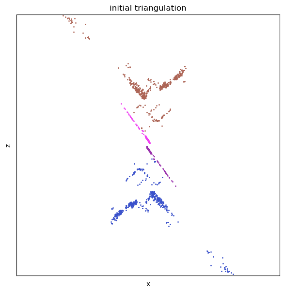
4.5. Triangulation Check for Cheirality Condition
In the previous section, we computed four different possible camera poses for a pair of images using essential matrix. In this section we will triangulate the 3D points, given two camera poses.
Given two camera poses, \((C_1, R_1)\) and \((C_2, R_2)\), and correspondences, \(x_1 \leftrightarrow x_2\), triangulate 3D points using linear least squares. Implement the function LinearTriangulation.py.
Though, in order to find the correct unique camera pose, we need to remove the disambiguity. This can be accomplished by checking the cheirality condition i.e. the reconstructed points must be in front of the cameras. To check the Cheirality condition, triangulate the 3D points (given two camera poses) using linear least squares to check the sign of the depth \(Z\) in the camera coordinate system w.r.t. camera center. A 3D point \(X\) is in front of the camera iff: \(r_3\mathbf{(X-C)} > 0\) where \(r_3\) is the third row of the rotation matrix (z-axis of the camera). Not all triangulated points satisfy this condition due of the presence of correspondence noise. The best camera configuration, \((C, R, X)\) is the one that produces the maximum number of points satisfying the cheirality condition.
Given four camera pose configurations and their triangulated points, find the unique camera
pose by checking the cheirality condition - the reconstructed points must be in front of the
cameras (implement the function DisambiguateCameraPose.py).
4.5.1. Non-Linear Triangulation
Given two camera poses and linearly triangulated points, \(X\), the locations of the 3D points that minimizes the reprojection error (Recall Project 2) can be refined. The linear triangulation minimizes the algebraic error. Though, the reprojection error is geometrically meaningful error and can be computed by measuring error between measurement and projected 3D point:
\(\underset{x}{\operatorname{min}}\) \(\sum_{j=1,2}\left(u^j - \frac{P_1^{jT}\widetilde{X}}{P_3^{jT}{X}}\right)^2 + \left(v^j - \frac{P_2^{jT}\widetilde{X}}{P_3^{jT}{X}}\right)^2\)
Here, \(j\) is the index of each camera, \(\widetilde{X}\) is the homogeneous representation of \(X\). \(P_i^T\) is each row of camera projection matrix, \(P\). This minimization is highly nonlinear due to the divisions. The initial guess of the solution, \(X_0\), is estimated via the linear triangulation to minimize the cost function. This minimization can be solved using nonlinear optimization functions such as scipy.optimize.leastsq or scipy.optimize.least_squares in Scipy library.
Given two camera poses and linearly triangulated points, \(X\), refine the locations of the 3D
points that minimizes reprojection error (implement the function NonlinearTriangulation.py).
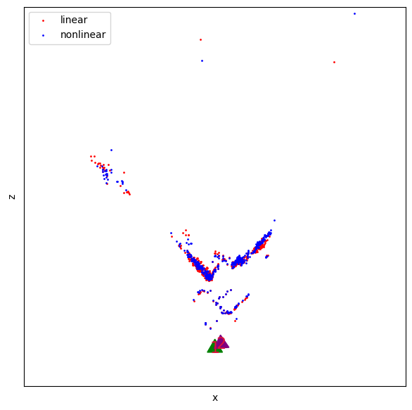
Once you implement both Linear and Non-linear triangulation, you can test if they are working by reprojecting the points of one image onto other using the estimated relative pose between them. They points should be closer in the non-linear triangulation method than the linear one (See Fig. 7).

4.6. Perspective-\(n\)-Points
Now, since we have a set of \(n\) 3D points in the world, their \(2D\) projections in the image and the intrinsic parameter; the 6 DOF camera pose can be estimated using linear least squares. This fundamental problem, in general is known as Perspective-\(n\)- Point (PnP). For there to exist a solution, \(n\geq 3\). There are multiple methods to solve the P\(n\)P problem and have an assumptions in most of them that the camera is calibrated. Methods such as Unified P\(n\)P (or UPnP) do not abide with the said assumption as they estimate both intrinsic and extrinsic parameters. In this section, you will a simpler version of PnP. You will register a new image given 2D-3D correspondences, i.e. \(X\leftrightarrow x\) followed by nonlinear optimization.
4.6.1 Linear Camera Pose Estimation
Given 2D-3D correspondences, \(X\leftrightarrow x\) and the intrinsic parameter \(K\), estimate the camera pose using linear least squares (implement the function LinearPnP.py. 2D points can be normalized by the intrinsic parameter to isolate camera parameters, \((C,R)\), i.e. \(K^{-1}x\). A linear least squares system that relates the 3D and 2D points can be solved for \((t, R)\) where \(t = −R^T C\). Since the linear least square solve does not enforce orthogonality of the rotation matrix, \(R \in SO(3)\), the rotation matrix must be corrected by \(R = UV^T\) where \(R=UDV^T\). If the corrected rotation has \(-1\) determinant, \(R = −R\). This linear PnP requires at least 6 correspondences. (Think why?)

4.6.2 PnP RANSAC
P\(n\)P is prone to error as there are outliers in the given set of point correspondences. To overcome this error, we can use RANSAC (yes, again!) to make our camera pose more robust to outliers. To formalize, given \(N \geq 6\) 3D-2D correspondences, \(X \leftrightarrow x\), implement the following function that estimates camera pose \((C, R)\) via RANSAC (implement the function PnPRANSAC.py).
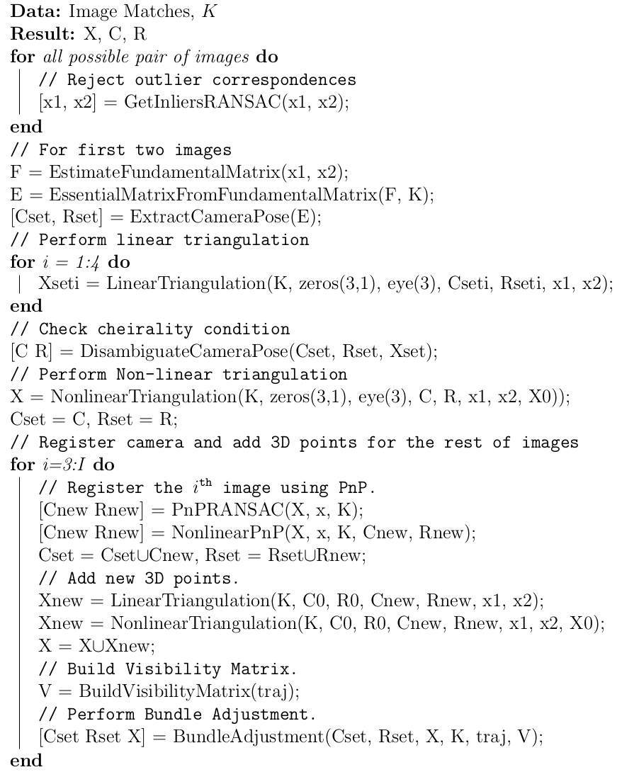
The alogrithm below depicts the solution with RANSAC.

Just like in triangulation, since we have the linearly estimated camera pose, we can refine the camera pose that minimizes the reprojection error (Linear PnP only minimizes the algebraic error).
4.6.3 Nonlinear PnP
Given \(N \geq 6\) 3D-2D correspondences, \(X \leftrightarrow x\), and linearly estimated camera pose, \((C, R)\), refine the camera pose that minimizes reprojection error (implement the function NonlinearPnP.py). The linear PnP minimizes algebraic error. Reprojection error that is geometrically meaningful error is computed by measuring error between measurement and projected 3D point
here \(\widetilde{X}\) is the homogeneous representation of \(X\). \(P_i^T\) is each row of camera projection matrix, \(P\) which is computed by \(P = KR [I_{3\times3} − C]\). A compact representation of the rotation matrix using quaternion is a better choice to enforce orthogonality of the rotation matrix, \(R = R(q)\) where \(q\) is four dimensional quaternion, i.e.,
\[\underset{C,q}{\operatorname{min}} \sum_{i=1,J} \left(u^j - \frac{P_1^{jT}\widetilde{X_j}}{P_3^{jT}{\widetilde{X_j}}}\right)^2 + \left(v^j - \frac{P_2^{jT}\widetilde{X_j}}{P_3^{jT}{X_j}}\right)^2\]This minimization is highly nonlinear because of the divisions and quaternion parameterization. The initial guess of the solution, \((C_0, R_0)\), estimated via the linear PnP is needed to
minimize the cost function. This minimization can be solved using a nonlinear optimization
function such as scipy.optimize.leastsq or scipy.optimize.least_squares in Scipy library.
4.7. Bundle Adjustment
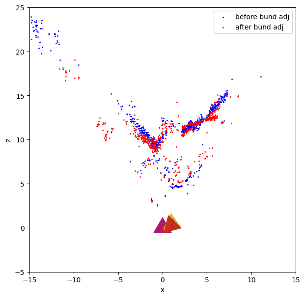
Once you have computed all the camera poses and 3D points, we need to refine the poses and 3D points together, initialized by previous reconstruction by minimizing reprojection error.
4.7.1 Visibility Matrix
Find the relationship between a camera and point, construct a \(I \times J\) binary matrix, \(V\) where
\(V_{ij}\) is one if the \(j^{th}\) point is visible from the \(i^{th}\) camera and zero otherwise (implement the
function BuildVisibilityMatrix.py)
4.7.2 Bundle Adjustment
Given initialized camera poses and 3D points, refine them by minimizing reprojection error (implement the function BundleAdjustment.py). The bundle adjustment refines camera
poses and 3D points simultaneously by minimizing the following reprojection error over \(C_{i_{i=1}}^I\),
\(q_{i_{i=1}}^I\) and \(X_{j_{j=1}}^J\).
The optimization problem can be formulated as following:
\(\underset{\{C_i, q_i\}_{i=1}^i,\{X\}_{j=1}^J}{\operatorname{min}}\sum_{i=1}^I\sum_{j=1}^J V_{ij}\left(\left(u^j - \dfrac{P_1^{jT}\tilde{X}}{P_3^{jT}\tilde{X}}\right)^2 + \left(v^j - \dfrac{P_2^{jT}\tilde{X}}{P_3^{jT}\tilde{X}}\right)^2\right)\) where \(V_{ij}\) is the visibility matrix.
Clearly, solving such a method to compute the structure from motion is complex and slow (can take from several minutes for only 8-10 images). This minimization can be solved using a nonlinear optimization functions such as scipy.optimize.leastsq but will be extremely slow due to a number of parameters. The Sparse Bundle Adjustment toolboxes such as large-scale BA in scipy and pySBA are designed to solve such optimization by exploiting sparsity of visibility matrix, \(V\) . Note that a small number of entries in \(V\) are one because a 3D point is visible from a small subset of images. Using the sparse bundle adjustment package is not trivial and would be much faster than one you write. For SBA, you are allowed to use any optimization library.
5. Putting the pipeline together
Write a program Wrapper.py that run the full pipeline of structure from motion based on the above algorithm.

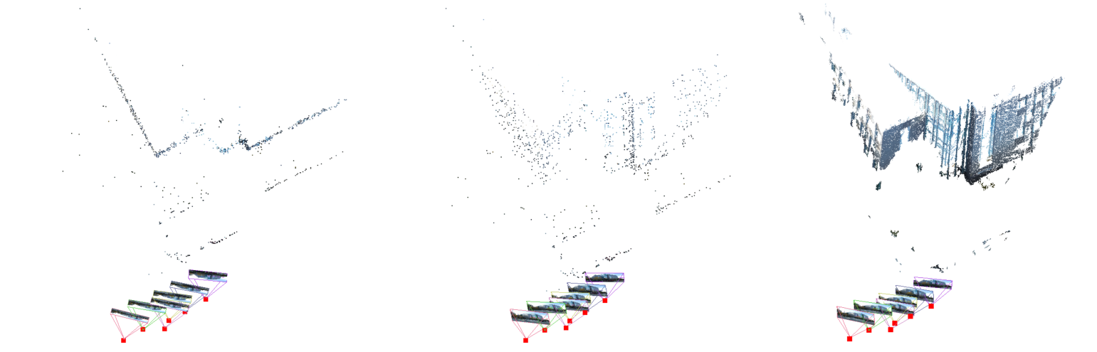
Also, you can compare your result against VSfM output. You can download the off-the-shelf SfM software here: VSfM. The output is shown below:
6. Phase: 2 Deep Learning Approach
You are going to be implementing the original NERF method (from this paper).
6.1 Dataset For NeRF
Download the lego data for NeRF from the original author’s link here. You are required to write your own data loader, parser, network and loss function for this phase.
6.2 Abstract and Method
NERF is a method that sparked a new revolution in the represention of 3D scenes by being able to synthesize novel views of complex scenes by optimizing an underlying continuous volumetric scene function using a sparse set of input views.

This approach represents a scene using a fully-connected (non-convolution) deep neural network, whose input is a single continuous 5D coordinate (spatial location (\(x, y, z\)) and viewing direction \(\theta, \psi\)) and whose output is the volume density and view-dependent emitted radiance at that spatial location.

They synthesize views by querying 5D coordinates along camera rays and use classic volume rendering techniques to project the output colors and densities into an image. Because volume rendering is naturally differentiable, the only input required to optimize our representation is a set of images with known camera poses. They describe how to effectively optimize neural radiance fields to render photorealistic novel views of scenes with complicated geometry and appearance, and demonstrate results that outperform prior work on neural rendering and view synthesis.
6.3 Synthetic Results
If you render a view to go around the Lego dataset, it should look like this:
You are required to produce an output like the one shown above.
7. Submission Guidelines
If your submission does not comply with the following guidelines, you’ll be given ZERO credit
7.1. File tree and naming
Your submission on ELMS/Canvas must be a zip file, following the naming convention YourDirectoryID_p3.zip. If you email ID is abc@wpi.edu, then your DirectoryID is abc. For our example, the submission file should be named abc_p3.zip. The submission must have the following directory structure because we’ll be autograding assignments. The file to run for your project should be called Wrapper.py. You can have any helper functions in sub-folders as you wish, be sure to index them using relative paths and if you have command line arguments for your Wrapper codes, make sure to have default values too. Please provide detailed instructions on how to run your code in README.md file. Please DO NOT include data in your submission.
YourDirectoryID_p3.zip
│   README.md
|   Your Code files
|   ├── Phase1/
|   | ├── GetInliersRANSAC.py
|   | ├── EstimateFundamentalMatrix.py
|   | ├── EssentialMatrixFromFundamentalMatrix.py
|   | ├── ExtractCameraPose.py
|   | ├── LinearTriangulation.py
|   | ├── DisambiguateCameraPose.py
|   | ├── NonlinearTriangulation.py
|   | ├── PnPRANSAC.py
|   | ├── NonlinearPnP.py
|   | ├── BuildVisibilityMatrix.py
|   | ├── BundleAdjustment.py
|   | ├── Wrapper.py
|   | ├── Any subfolders you want along with files
|   | Wrapper.py
|   | Data
|   | └── IntermediateOutputImages/
|   └── Phase2/
|     ├── All Codes For NeRF
|     └── NeRF.gif
└── Report.pdf
7.2. Report
There will be no Test Set for this project. For each section of the project, explain briefly what you did, and describe any interesting problems you encountered and/or solutions you implemented. You must include the following details in your writeup:
-
Please make your report extremely detailed with re-projection error (in a table form and show images with reprojections) after each step in Phase 1 (Linear, Non-linear triangulation, Linear, Non-linear PnP before and after BA and so on). Describe all the steps (anything that is not obvious) and any other observations in your report.
-
For Phase 2, show results of novel views (take frames from the gif you created). Talk about any issues you faced and how you solved them.
-
Your report MUST be typeset in LaTeX in the IEEE Tran format provided to you in the
Draftfolder and should of a conference quality paper. -
Present failure cases and explanation, if any.
-
Do not use any function that directly implements a part of the pipeline. If you have any doubts, please contact us via Piazza.
8. Extra Credit
8.1. Phase 1
- Collect your own data and run your SfM code. The following tips should help your chances of success:
- Collect your data in PRO mode with all settings fixed manually (including focus, use manual focus)
- Collect data of your object of interest (building for example) in neutral lighting (like dawn or dusk or cloudy days)
- Calibrate your camera with same focus and setting you collected your data from using any calibration target/toolbox (If you are resizing the images for processing, calibrate after resizing the calibration images using the same settings)
- Use undistorted images (from your calibration data) and find feature matches (Use SIFT with a high sensitivity, I have not found other “faster” features to not work well)
- Run your code to obtain SfM outputs
- Experiment with other feature detectors and descriptors including deep learning ones. Here’s a good reference to use/learn about these.
8.2. Phase 2
- Collect your own data and run your NeRF code. The following tips should help your chances of success:
- Collect data for NeRF similar to SfM (as decribed in the previous subsection) with the difference being that you need to go around the entire object (make sure that the object has a matte texture with almost no reflections)
- Make sure your scene has uniform soft lighting
- Make sure to have black or white background
- Obtain Ground Truth poses using COLMAP or VisualSfM
- Train your NeRF network and present results
If any of these are implemented, also place your input images (for Phase 1) and sample dataset images (for Phase 2) along with link to download these images with final results in your report PDF.
Implement the any or all of the above methods to earn upto 25% extra credit (when everything is implemented).
9. Collaboration Policy
You are encouraged to discuss the ideas with your peers. However, the code should be your own, and should be the result of you exercising your own understanding of it. If you reference anyone else’s code in writing your project, you must properly cite it in your code (in comments) and your writeup. For the full honor code refer to the RBE/CS549 Full 2022 website.
10. Acknowledgments
This fun project was inspired by a similar project in UPenn’s CIS581 (Computer Vision & Computational Photography), University of Maryland’s CMSC733 (Classical and Deep Learning Approaches for Geometric Computer Vision) and Carnegie Mellon University’s 16-889 (Learning for 3D Vision).