Deep and Un-Deep Visual Inertial Odometry
Table of Contents:
- 1. Deadline
- 2. Introduction
- 3. Phase 1: Classical Visual-Inertial Odometry
- 4. Phase 2: Deep Visual-Inertial Odometry
- 5. Expected Output
- 6. Submission Guidelines
- 7. Allowed and Disallowed functions
- 8. Collaboration Policy
1. Deadline
11:59:59 PM, April 14, 2023 and 11:59PM, April 28, 2023. This project is to be done in groups of 2 and has a 10 min presentation. Various checkpoints are due at different dates and are given below:
- Checkpoint 1 is due on 11:59:59 PM, April 14, 2023.
- Checkpoint 2 is due on 11:59:59 PM, April 28, 2023.
You cannot use any LATE days for this assignment.
2. Introduction
As we have talked about multiple times in class, it is impossible to obtain scale from a single camera without some prior information. Although, you might be wondering well a deep network can do it without any knowledge - it is not quite true! The prior in this case comes from the data that was used to train the network. Furthermore, keen readers might have realized that it will not work when a new “out of domain” data is presented, for e.g., if you train on indoor images and show an outdoor image with no indoor objects. It will not work! One way to get around this is by training on a huge dataset with almost everything one might see. This is hard and not scalable! A much simpler solution is to utilize a stereo camera with known distance (more generally, the pose) between cameras. In this case one would directly obtain depth by matching features! Great! So is it all solved then? Not at all, first of all matching is expensive and hard, secondly, this does not work when there is motion blur which is common on robots! How do we solve this? We can utilize a cheap sensor which is almost always present on robots - an Inertial Measurement Unit (IMU). A common 6-DoF (Degree of Freedom) IMU measures linear acceleration and angular acceleration. The best part about an IMU is that it works well with fast movement and jerks where camera fails but drifts over time in which camera excels. Hence, this complementary nature lends to a beautiful multi-modal fusion problem which can be used to estimate accurate pose of the camera to backtrack depth! Now using this methodology our robots can operate in high-speed and wild conditions! Awesome right? Indeed, this was used in the DARPA Fast Light Autonomy (FLA) project where a team from Vijay Kumar’s Lab at University of Pennsylvania achieved 20m/s autonomous flight using a VIO approach. You can watch the video here. As a side note, if you have no idea about an IMU, I have some tutorials that cover the basics of IMUs here.
This project is in two phases, in the first phase, you will implement a classical approach for Visual-Inertial fusion to obtain odometry. The second phase is open-ended, where you will formulate an approach to perform Visual-Inertial (VI) fusion using deep learning.
3. Phase 1: Classical Visual-Inertial Odometry
Your goal in this phase is to implement the following paper which we talked about before. You might also need to refer to the seminal VIO paper using MSCKF to understand the mathematical model. Since it is a complicated method, you are required to only implement a few functions in the starter code provided. We’ll describe the data and the codebase next.
3.1. Data
We will be using the Machine Hall 01 easy or (MH_01_easy) subset of the EuRoC dataset to test our implementation. Please download the data in ASL data format from here. Here, the data is collected using a VI sensor carried by a quadrotor flying a trajectory. The ground truth is provided by a sub-mm accurate Vicon Motion capture system.
We will talk about the starter code next.
3.2. Starter Code
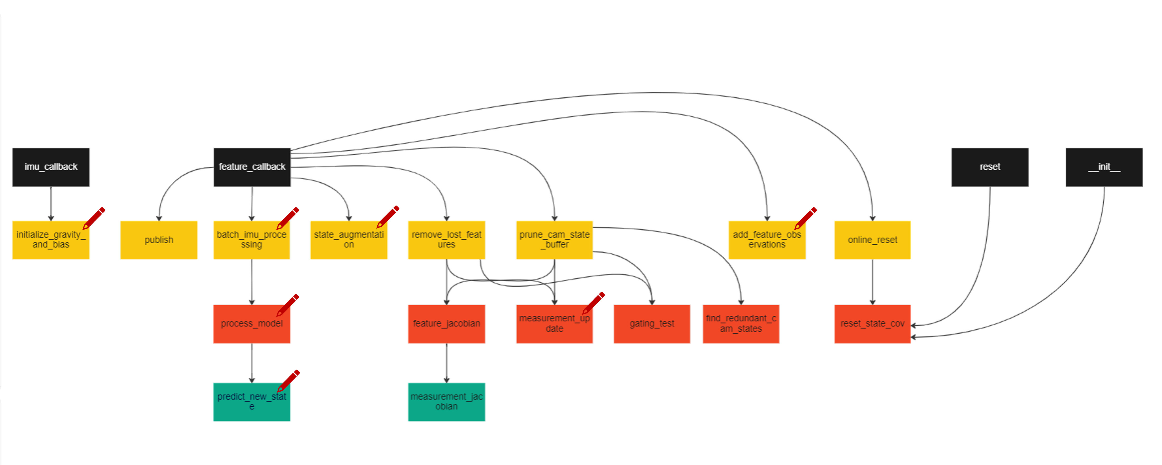
The starter code can be downloaded from here. It contains the Python implementation of the C++ code provided by the authors of S-MSCKF paper here. You will be implementing eight functions in the msckf.py file. Please refer to README.md file for instructions on how to run the code with and without visualization along with the package requirements. Specifically, you’ll be implementing the following functions: initialize_gravity_and_bias (estimates gravity and bias using initial few measurements of IMU), batch_imu_processing (Processes the messages in the imu_msg_buffer, executes the process model and updates the state), process_model (Dynamics of the IMU error state), predict_new_state (Handles the transition and covariance matrices), state_augmentation (Adds the new camera to state and updates), add_feature_observations (Adds the image features to the state), measurement_update (Updates the state using the measurement model) and predict_new_state (Propogates the state using 4th order Runge-Kutta). More detailed and step by step comments are given in the starter code. The strtcure of the code is based on how it would be performed in Robot Operating System (ROS) and function callbacks and might be confusing for someone who has never used networking or ROS before. Do ask us questions if you do not understand the codebase. The structure of the msckf.py file you need to modify is shown in Fig. 1, where a red pencil icon indicates that you need to implement that function.
4. Phase 2: Deep Visual-Inertial Odometry
Once you finish the implementation of the previous stage, you might have realized that the classical approach relies heavily on feature detection and tracking. You might be thinking, why cannot we simply replace it deep feature matching such as SuperPoint or SuperGlue? Yes, indeed this would work. But similar set of features are hard to conceptualize for inertial data. Although there have been some great works on Inertial navigation, only a few works tackle VI-fusion using deep learning. In this phase, you will “come-up” with an architecture, loss function and methodology (you are free to adapt from earlier works) to predict relative pose between two image frames along with IMU measurements. To summarize, input is two image frames along with all IMU measurements between and the output is relative pose between two camera frames.
4.1. Data
We will be using the Machine Hall 02 easy (MH_02_easy), Machine Hall 03 medium (MH_03_medium), Machine Hall 04 difficult (MH_04_difficult) and Machine Hall 05 difficult (difficult) subsets of the EuRoC dataset for training the neural network. Present your results on Machine Hall 01 easy (MH_01_easy) subset of the EuRoC dataset. Feel free to download the data in any format and utilize any code for data handling and processing. Here, the data is collected using a VI sensor carried by a quadrotor flying a trajectory. The ground truth is provided by a sub-mm accurate Vicon Motion capture system.
5. Expected Output
5.1. Phase 1
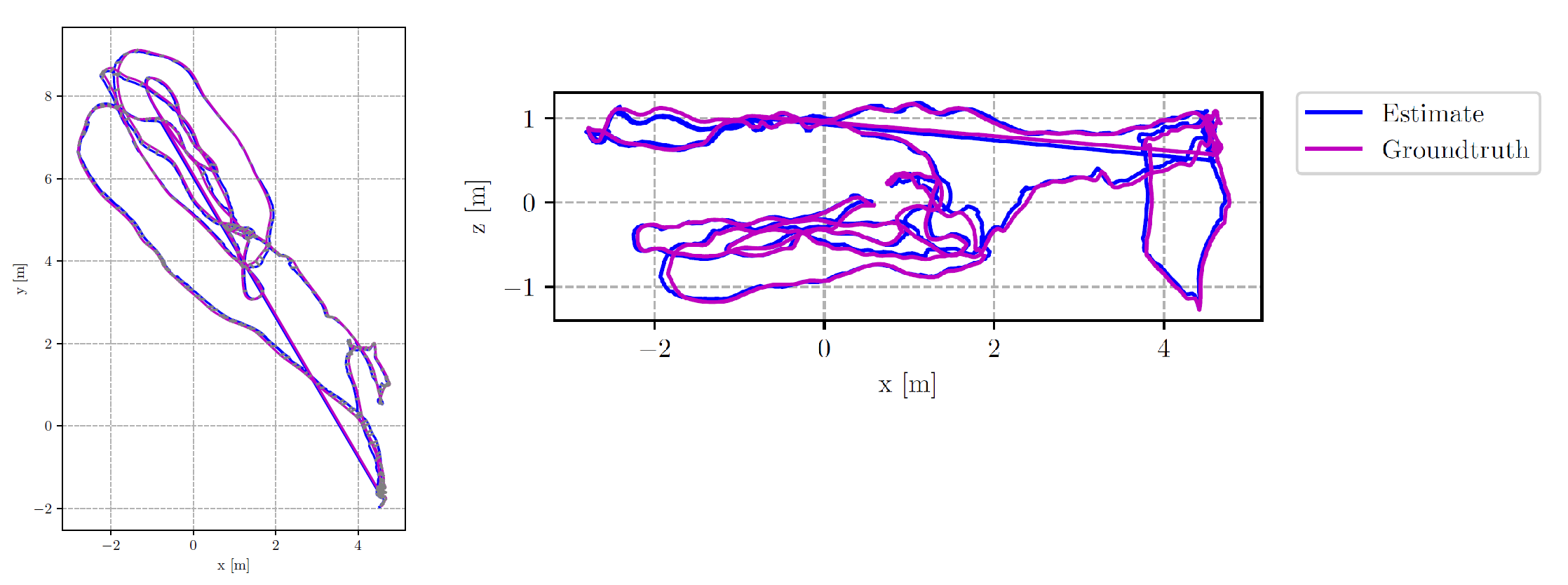
The output for Phase 1 is from the code visualization is shown in Fig. 2. But you have to plot the ground truth in “red/pink” color alongside your trajectory estimates (in black/blue) and compute error as shown in Fig. 3. Given your predictions and the ground truth from Vicon, compute the RMSE ATE error using any toolbox you like. You might have to perform an SE(3) alignment before computing error. Refer to this toolbox for details and implementation. Mention this error in your report. In addition to RMSE ATE, feel free to also compute error using any other metrics and mention them in your report. Also, present a screen capture of your code running with trajectory being visualized as Output.mp4.

5.2. Phase 2
Just like the last phase, you are expected to show a plot of the ground truth trajectory and it’s evaluation along with the predictions from your neural network. Present and compare results from the output of the previous phase, vision data only (training and predictions with only two images as the input, see Fig. 4a), inertial data only (training and predictions with only IMU data as the input, see Fig. 4b) and finally visual-inertial data predictions (training and predictions with two images and inertial data between them as the input, see Fig. 4c).

6. Submission Guidelines
If your submission does not comply with the following guidelines, you’ll be given ZERO credit
6.1. File tree and naming
Your submission on ELMS/Canvas must be a zip file, following the naming convention YourDirectoryID_p4.zip. If you email ID is abc@wpi.edu, then your DirectoryID is abc. For our example, the submission file should be named abc_p4.zip. The submission must have the following directory structure. The file vio.py is expected to run using the command given in the README.md file for phase 1. You can have any helper functions in sub-folders as you wish, be sure to index them using relative paths and if you have command line arguments for your Wrapper codes, make sure to have default values too. Please add to any further instructions on how to run your code in README.md file. Please DO NOT include data in your submission.
YourDirectoryID_p4.zip
│   README.md
|   Code
|   ├── Phase 1
|   | ├── All given code files
|   | └── Any subfolders you want along with files
|   └── Phase 2
|     └── Any subfolders you want along with files
├── Output.mp4
└── Report.pdf
6.2. Report
For each section and phase of newly developed solution in the project, explain briefly what you did, and describe any interesting problems you encountered and/or solutions you implemented. You must include the following details in your writeup:
- Your report MUST be typeset in LaTeX in the IEEE Tran format provided to you in the
Draftfolder and should of a conference quality paper. - Brief explanation of your approach to this problem. Talk about all the equations you used to implement the parts of code requested (eight functions).
- Present a plot comparison of your estimated trajectory (any color except red) along with Vicon ground truth (in red) for phase 1.
- Comparison of predictions of vision only, inertial only, visual-inertial in phase 2 and comparison to phase 1.
- RMSE ATE error of your estimated trajectory with respect to Vicon for both phases.
- Any other error metrics you used along with their error values.
- Any key insights into the problem of VIO.
- Present what research problems you can work on for both classical and deep VIO approaches. This is super important!
6.3 Video
Screen capture of your code running with trajectory being visualized as Output.mp4.
6.4. Presentation
You are required to do an in-person presentation for 10mins (all team members MUST present) during the time decided (look out for a post on timings on Piazza) explaining your approach, the results as video. Explain what all problems you tackled during this project and how you overcame them. Further, talk about non-obvious observations, corner cases and failure modes along with potential ways to solve them. Also, give an in-depth analysis of your proposed approach. The presentation has to be professional of a conference quality presented to a wide range of audience ranging from a lay-person to an expert in the field.
7. Allowed and Disallowed functions
Allowed:
- Basic math functions from numpy and scipy along with packages given in starter code for Phase 1.
- Any dataloader and other helper functions required to implement phase 2.
Disallowed:
- Things that directly implement parts of phase 1.
- Things that implement architecture or loss function (unless built-in into PyTorch) for phase 2.
If you have any doubts regarding allowed and disallowed functions, please drop a public post on Piazza.
8. Collaboration Policy
You are encouraged to discuss the ideas with your peers. However, the code should be your own, and should be the result of you exercising your own understanding of it. If you reference anyone else’s code in writing your project, you must properly cite it in your code (in comments) and your writeup. For the full honor code refer to the RBE/CS549 Full 2023 website.